Metasample annotation using BIODICA
Altynbek Zhubanchaliyev, Nicolas Captier
The aim of this tutorial is to demonstrate how BIODICA can find associations between features from annotation files and metasamples associated with identified stabilized Independent Components (IC’s). We will use 30 IC’s extracted from OVCA-transcriptomic dataset in the ICA decomposition tutorial.
Warning : When running this tutorial, please keep in mind that the ranking of the IC’s will not necessarily be the same as indicated here, since BIODICA uses ICA decomposition algorithm with random initializations. For instance, IC21 we refer to in this tutorial may correspond to an IC with a ranking other than 21 in your case.
Running metasample annotation analysis
-
Open Metasample Annotation

-
Specify a metasample table A (e.g. BIODICA/work/OVCA_ICA/OVCA_ica_A.xls) and a sample annotation file (e.g. BIODICA/data/OVCA_TCGA/sample_info/OVCA_samples_annotations.txt). This file should contain in rows the same samples as your original data set and in columns additional features (e.g. “age_at_diagnosis”, “overall_survival”…). The first row always lists feature names and the first columns always contains sample ids. The first column should have a name as well.

Warning : Ids of the samples in the sample annotation file should match exactly the sample names in the original omics data set. This is important to check in advance. -
Click on ‘Run’. The analysis process will finish quickly. The web-browser tab will open. It may take some time since BIODICA has to process all the generated files into one html report. It will look like this :
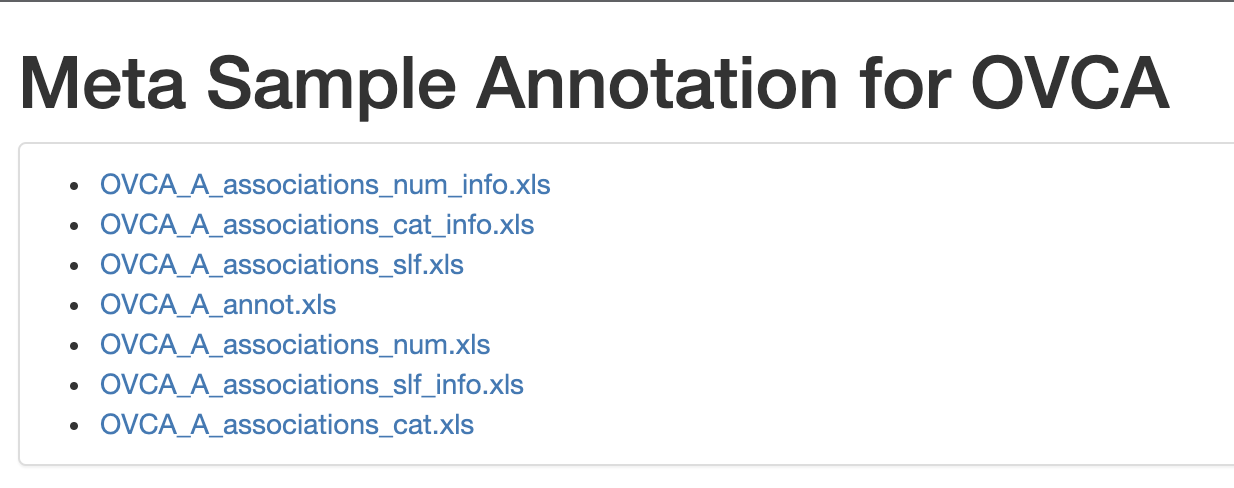
It contains the summary of all the associations, and the user can download each of the files directly from the web-browser, by clicking on the file name (e.g. OVCA_A_annot.xls). The files are stored in the newly created directory (BIODICA/work/OVCA_MSAMPLE).
Annotation results
In the sample annotation file, all sample features are classified into numerical and categorical. The feature is considered categorical if it contains non-numerical symbols as values, or if the number of distinct numerical values is less than minNumberOfDistinctValuesInNumericals BIODICA parameter. All missing values (marked by “NA” or “_”) are ignored.
Note : By default minNumberOfDistinctValuesInNumericals BIODICA parameter is set to 10. We will see how to change it at the end of the tutorial.
Categorical features
If the sample feature is categorical, and the number of categories is less than MaxNumberOfCategories parameter, then the association is computed by calculating the p-value of the Wilcoxon test between all pairs of categories and metasample weights. If in the pair, one of the categories is represented by less than minNumberOfSamplesInCategory samples then the test is not computed. The minimum p-value between all pair-wise comparisons is assigned to the association test between a sample feature and an independent component represented as a metasample.
Note : By default MaxNumberOfCategories and minNumberOfSamplesInCategory BIODICA parameters are set to 10 and 3. We will see how to change them at the end of the tutorial.
The –log10(p-value) values are reported in the association table. Those sample features which are not associated to any independent component are not reported in the association table.
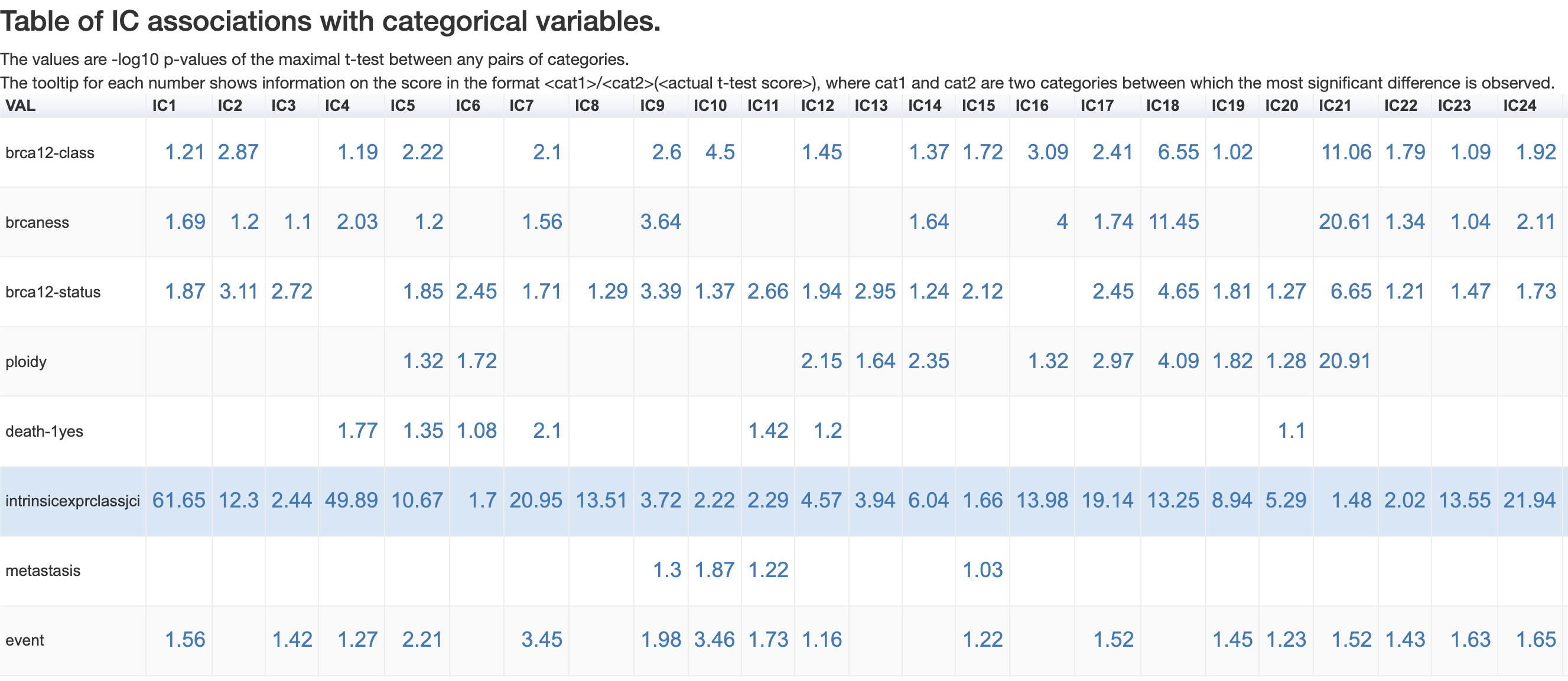
For instance, IC21 recieved significant associations with features of ‘brcaness’ (p-value = 10 ** -20.61) and ‘ploidy’ (p-value = 10 ** -20.91).
-
Let us now click on the number 20.61, IC21 ‘brcaness’. The following graph shows in more detail how the categories of ‘brcaness’ are different for IC21 metasample weights. Both categories have a sufficient sample size, and the difference between means of the groups is significant.

-
Let us now look at the association between IC4 and ‘intrinsicexprclassjci’ with -log10 p-value of 49.89. When we hover the mouse over the number 49.89, it shows the pair of categories between which the most significant difference is observed (the value of the associated t-test is shown as well).

-
Let us now click on the number and open the charts. We do observe that proliferative and immunoreactive groups have the largest difference. The graph is interactive and you can look at different parameters of the distribution.

Numerical features
If the sample feature is truly numerical then the association is computed by calculating the Spearman correlation coefficient between the feature and the metasample weights.
The correlation coefficients are reported in the association table. The number which appears after you hover your mouse on it corresponds to the associated -log10(p-value).
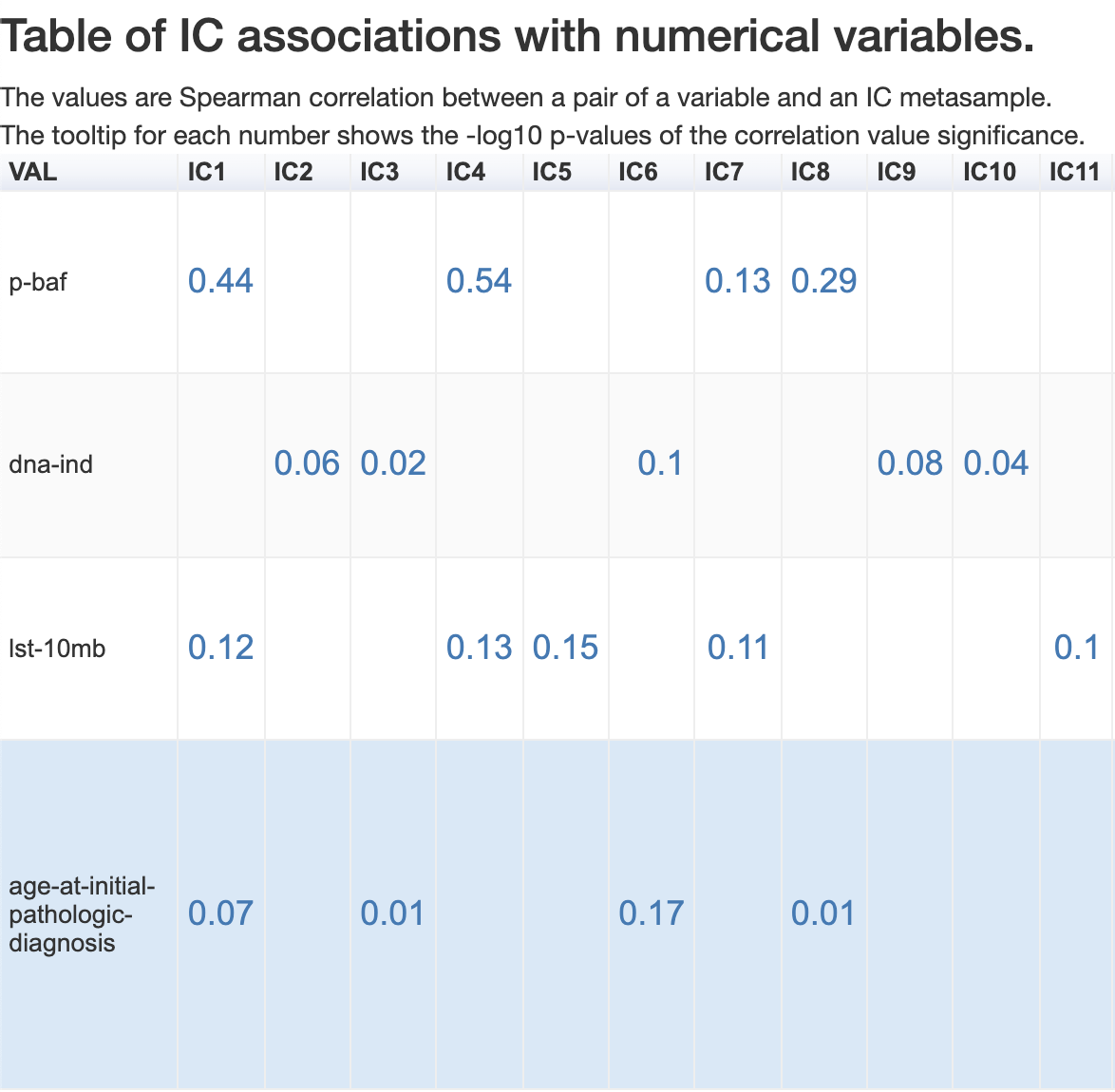
Let us click on the age-at-initial-pathologic-diagnosis of IC17, which has a Spearman correlation coefficient 0.29. We will see the following distribution :

IC associations with themselves
Finally, we can observe the Spearman coefficient correlation for each pair of IC metasamples.
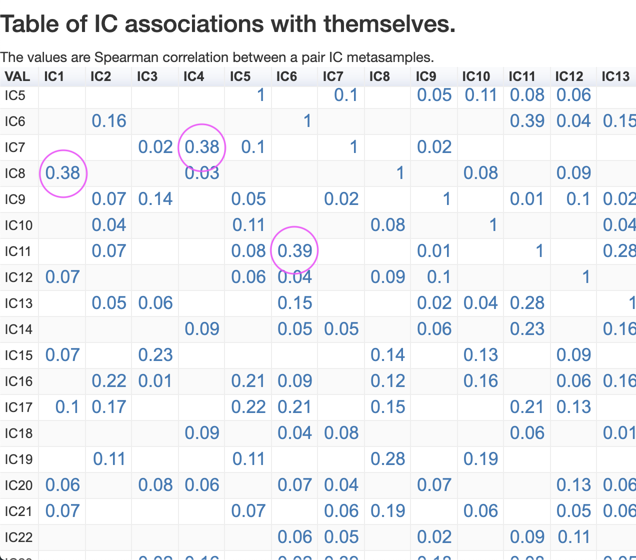
For instance, IC6 and IC11 have a correlation 0.39, which is among the highest in this dataset. IC23 and IC30 have a correlation 0.52.
Change analysis parameters values
In the Parameters menu, go to the Analysis parameters tab and change the analaysis paramaters.
