ICA decomposition using BIODICA Navigator
Altynbek Zhubanchaliyev, Nicolas Captier
In recent years stabilized Independent Component Analysis (ICA), a method of matrix factorization, has shown itself as a promising and reliable tool to obtain reproducible results in the task of feature extraction from transcriptomics data (Cantini et al., 2019; Aynaud et al., 2020). BIODICA offers an easy-to-use graphical tool to run a python implementation of stabilized ICA (available in the package stabilized-ica) for omics datasets.
This tutorial aims to demonstrate how to use BIODICA and perform stabilized ICA on the test OVCA-TCGA transcriptomic dataset (available in BIODICA).
Initial steps
Launching BIODICA
After cloning BIODICA into your local folder, launch it from inside the folder by running:
java -jar BIODICA_GUI.jar. It is important that your current directory is the BIODICA folder, and you are not launching it from an absolute path.
Note : In this tutorial the name of our folder is ‘BIODICA’. Do not use spaces and hyphens in the name, if you rename it.
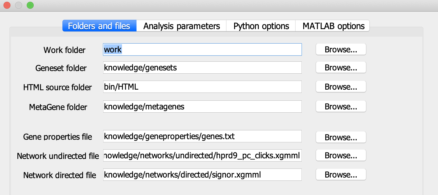
Choosing a work folder
Click on ‘Parameters’ and choose the working folder, where your results will be saved. By default it is ‘work’ folder (BIODICA/work).

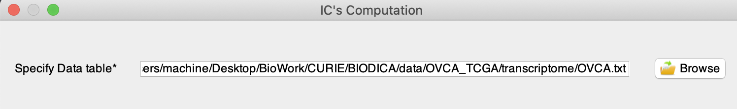
Loading a dataset
Close the parameters window and clik on ‘Run ICA’. Specify the input data table by clicking on ‘Browse’ or by writing a path to access your dataset. For this tutorial, we will use OVCA-TCGA dataset in (BIODICA/data/transcriptome/OVCA.txt).
General recommendations on the data format for BIODICA:
- Dataset should be a tab-delimited matrix
- Genes as rows, samples as columns (rows could be proteins, methylation sites, or other measured signals)
- Gene names should be in HUGO format
- For transcriptomics studies we recommend centering the expression of each gene as a pre-processing step
Running stabilized ICA
In the Parameters of ICA method section you will see four options. The first two specify the way to apply stabilized ICA to your dataset. You can either perform ICA decomposition for a single fixed number of components or for a range of different numbers of components. The last two options are only available once ICA decomposition has already been performed for this dataset. We will deal with them in the next section.
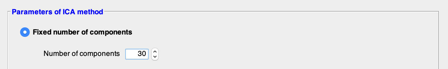
ICA with fixed number of components
-
Select the option Fixed number of components and choose the number of independent components you want to decompose your data into. For our tutorial, we choose the fixed number of 30 components as it provides a satisfying trade-off between a high overall component stability and a sufficiently large number of components to capture the underlying information present in our input data.
-
Click on ‘Run’
We obtain two matrices: matrix_A - containing 30 metasamples, and matrix_S - containing 30 metagenes. Metagene refers to a set of numerical weights (positive or negative) associated to each gene in the input dataset. They correspond to the projection of each gene on the associated independent component. Metasample refers to a set of numerical weights (positive or negative) associated to each sample in the input dataset. They correspond to the projection of each sample on the associated independent component. Both matrices are stored in the corresponding .xls files, in our (work/OVCA_ICA) directory.
Alternatively, we can download them directly from html tab in web-browser, by clicking on each matrix file, as indicated below:

If the web-browser tab didn’t open after you run the ICA, click on ‘Open results’ at the bottom of the window, and then ‘OK’. It will open the web-browser tab with results.

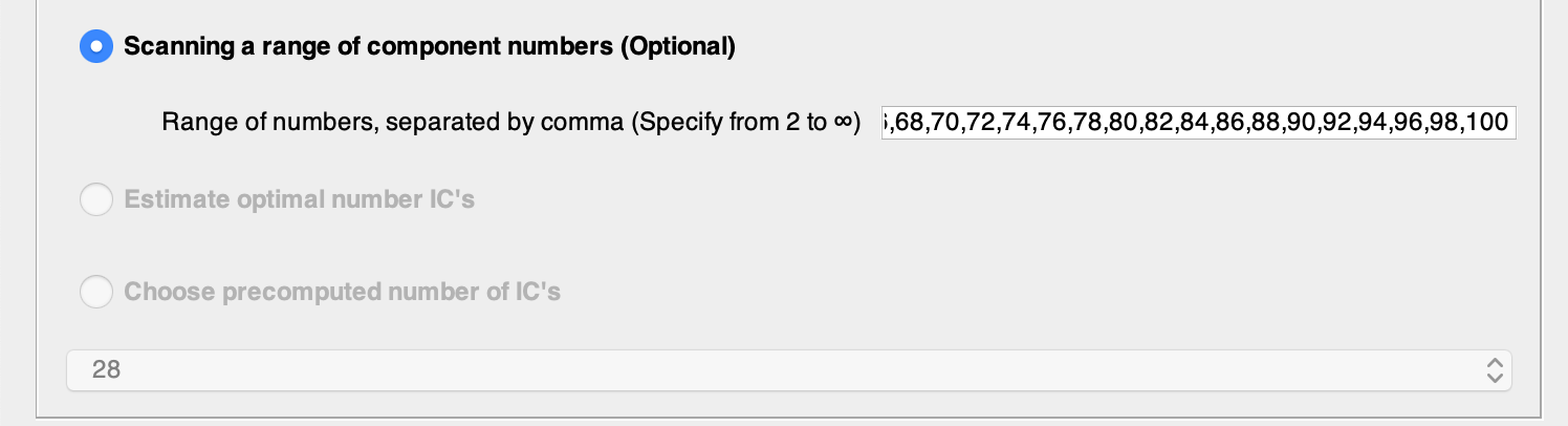
ICA with a range of different numbers of components
-
Choose ‘Scanning a range of components number’ and write the different numbers separated by comma (without spaces). For this tutorial we will use every even number from 4 to 100. Scanning range is needed for further estimation of the optimal number of components.
-
Click on ‘Run’. This will activate the process and you will get the message.

-
Click on ‘OK’. This creates result files in your ‘work’ directory and opens a tab in the web-browser with stability graph and umap figure of the components.
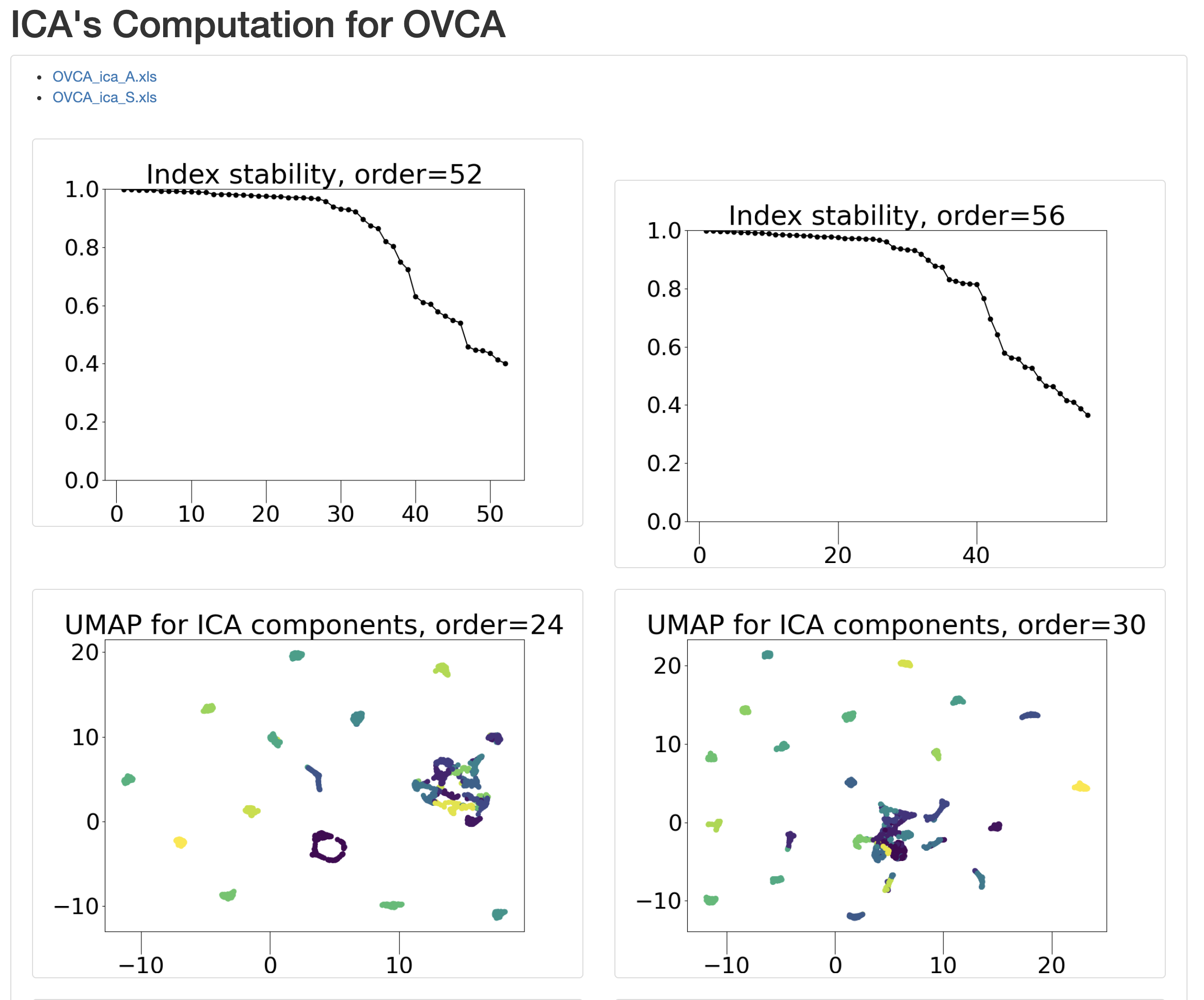
For instance ‘Index stability, order = 52’ indicates stability indices of each of the components for ICA with 52 IC’s.
Using pre-computed ICA decompositions
BIODICA will store all the results of ICA computation for all of the numbers of IC’s that you have performed for this dataset. You can easily access them with the Choose precomputed number of IC’s option or perform a meta-analysis to estimate a relevant order of decomposition with the Estimate optimal number of IC’s option.
ICA with precomputed number of components
-
Select an order of decomposition you want to access and that has already been computed. In this tutorial we choose 18 for demonstration.

-
Click on ‘Run’. A message saying that ICA for 18 components is successful appears, click on ‘OK’ and then on ‘Open results’.
Now are our OVCA_ica_A.xls and OVCA_ica_S.xls matrices contain results for 18 independent components.
Estimate an optimal number of IC’s
-
Select the ‘Estimate optimal number of IC’s’ option.

-
Click on ‘Run’.
We get the ‘Index of stability’ graph for all the number of components we have computed and the Mean Stability graph, that look like this.
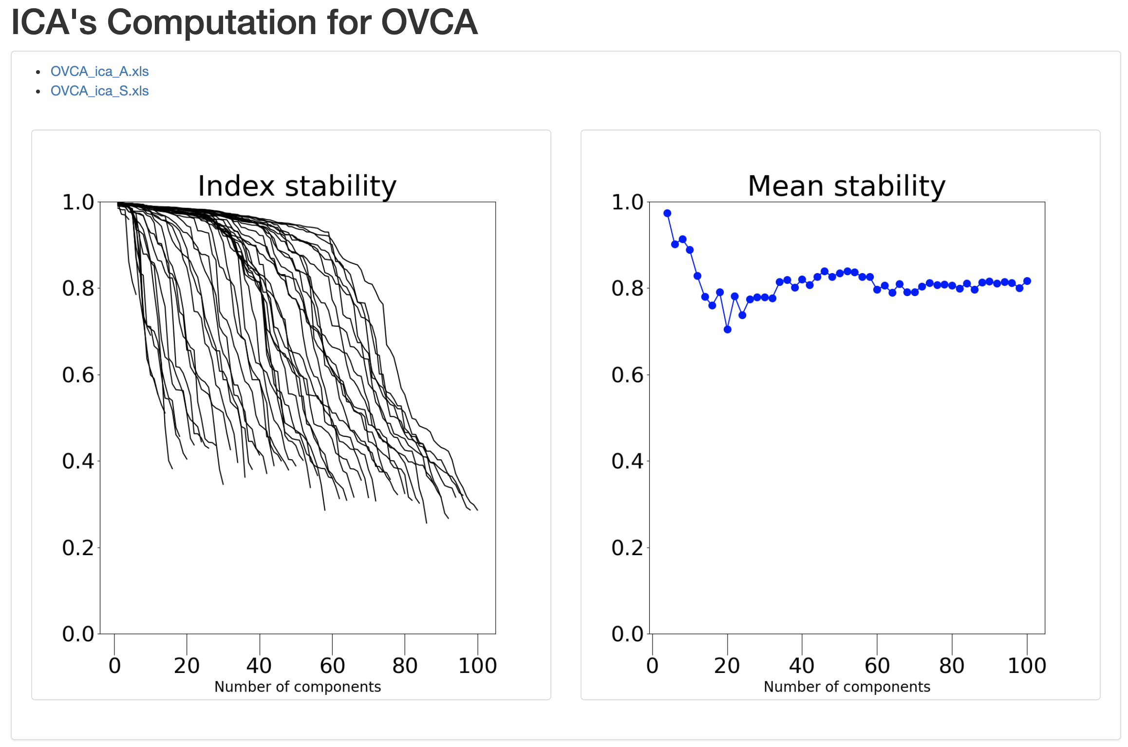
These graphs will help the user select a number of components which realizes a satisfying trade-off between a sufficiently large number of components to capture the information present in the input dataset and a high overall stability to ensure reproducible ICA components.
Note : The Estimate optimal number of IC’s option will not give you a single order of decomposition. It will rather give you tools to select yourself a relevant order of decomposition following the philosophy “not too few components, not too many instable components”. This choice is very much data-, application-, but also user-dependent.
Additional remarks
-
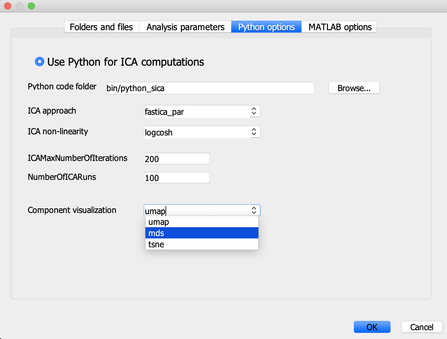
There is an option to choose graphical representations of IC’s other than umap, e.g. mds. In the Parameters menu, and Python options select ‘Component visualization’.
-
You can copy and paste this line into the Scanning a range of component numbers option.
4,6,8,10,12,14,16,18,20,22,24,26,28,30,32,34,36,38,40,42,44,46,48,50,52,54,56,58,60,62,64,66,68,70,72,74,76,78,80,82,84,86,88,90,92,94,96,98,100
This will give a good range of components to estimate an optimal one. Click on Estimate number of components and look at the graphs.