Metagene annotation using BIODICA
Altynbek Zhubanchaliyev, Nicolas Captier
The aim of this tutorial is to demonstrate how BIODICA can find associations between gene properties (numerical and categorical) and metagenes associated with identified stabilized Independent Components (IC’s). We will use 30 IC’s extracted from OVCA-transcriptomic dataset in the ICA decomposition tutorial.
Warning : When running this tutorial, please keep in mind that the ranking of the IC’s will not necessarily be the same as indicated here, since BIODICA uses ICA decomposition algorithm with random initializations. For instance, IC5 we refer to in this tutorial may correspond to an IC with a ranking other than 5 in your case.
Running metagene annotation analysis
-
Open Metagene Annotation

-
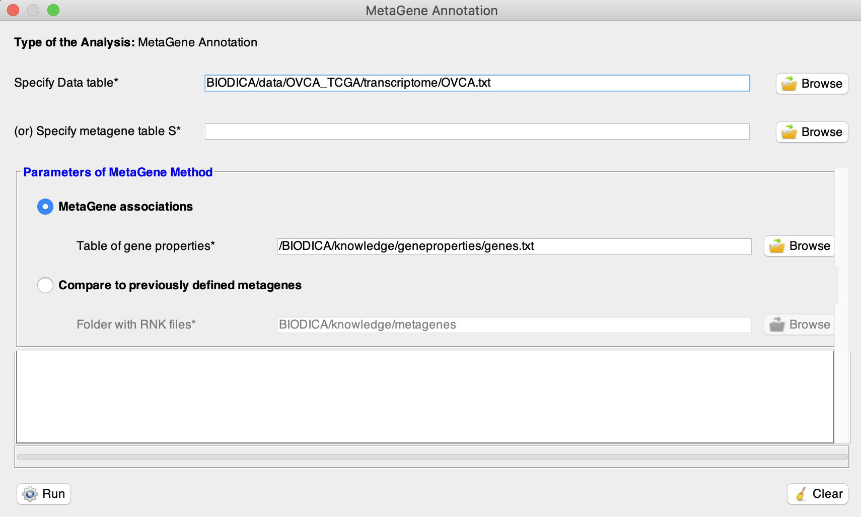
Specify Data table (e.g. BIODICA/data/OVCA_TCGA/transcriptome/OVCA.txt).
-
First, run the MetaGene Annotation with the selected option ‘Metagene associations’ (BIODICA/knowledge/geneproperties/genes.txt). The web-browser tab will open. You can close it.
-
Then run the MetaGene Annotation with an option ‘Compare to previously defined metagenes’ (BIODICA/knowledge/metagenes).
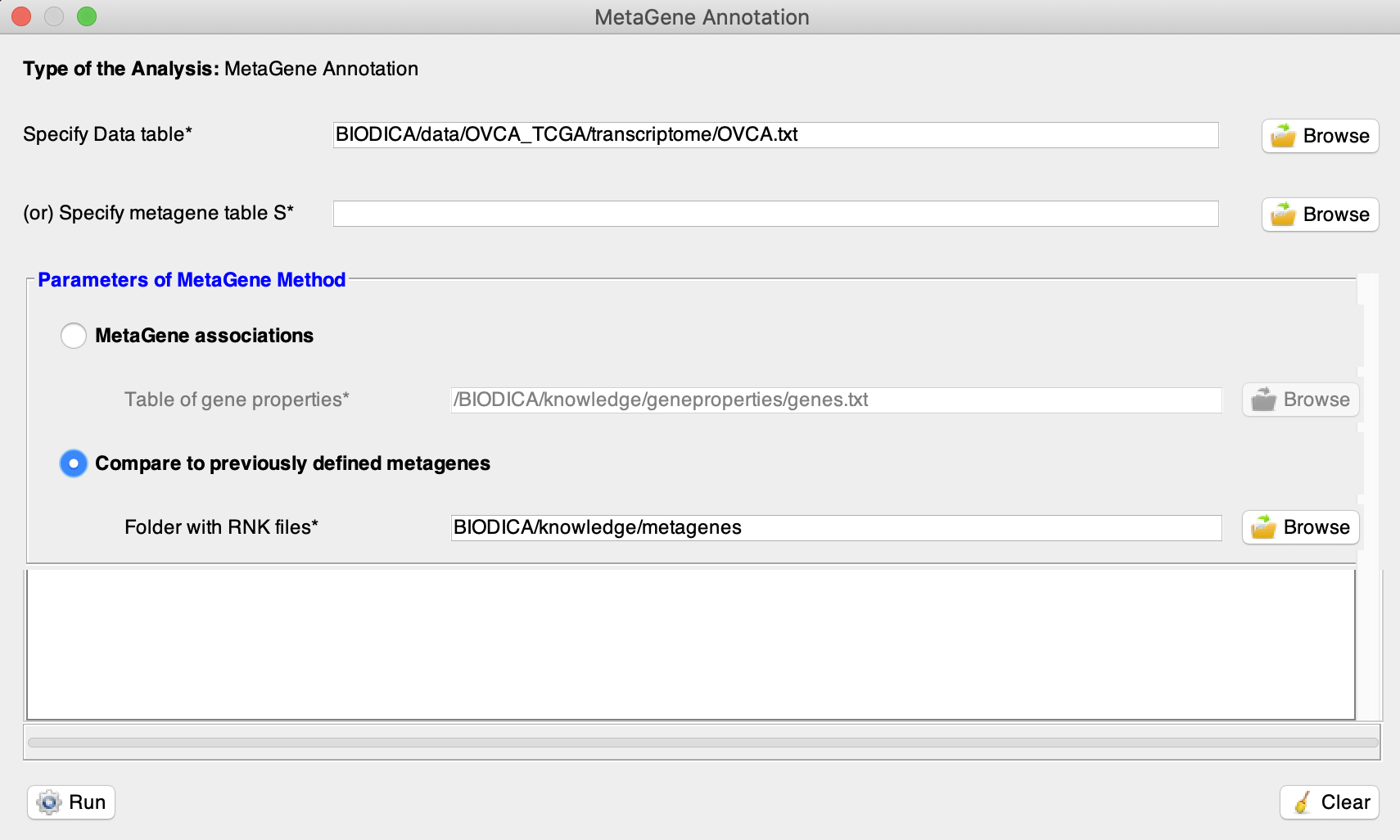
Note : We can load any previously defined metagenes. The folder should contain one .rnk file for each metagene. Each file should contain two columns, the first one with the gene names and the second one with the associated gene weights. See the BIODICA/knowledge/metagenes folder for more details.
The MetaGene Annotation web-browser tab will open. It may take some time since BIODICA has to process all the generated files into one html report. It will look as follows :
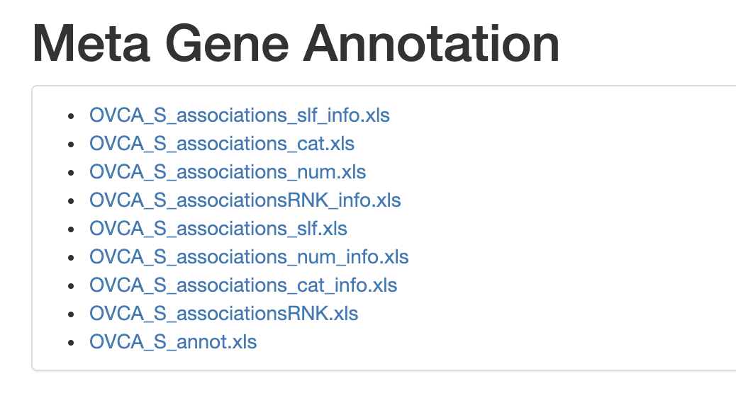
The files are stored in the newly created directory (BIODICA/work/OVCA_MGENE).
Annotation results
For the association of the metagenes with gene annotations, either categorical ones or numerical ones, BIODICA uses the same method as the one used for the metasample annotation.
Association with categorical features
For a categorical gene annotation, its association with a metagene is computed by calculating the p-value of the Wilcoxon test between all pairs of categories and the metagene weights. The minimum p-value between all pair-wise comparisons is assigned to the association test.
Inside the categorical gene annotation TYPE we have several categories describing the origin of the transcript (e.g. protein_coding, lncRNA, snoRNA…). The –log10(p-value) values of the associations between each metagene and the gene feature TYPE are reported in the association table.
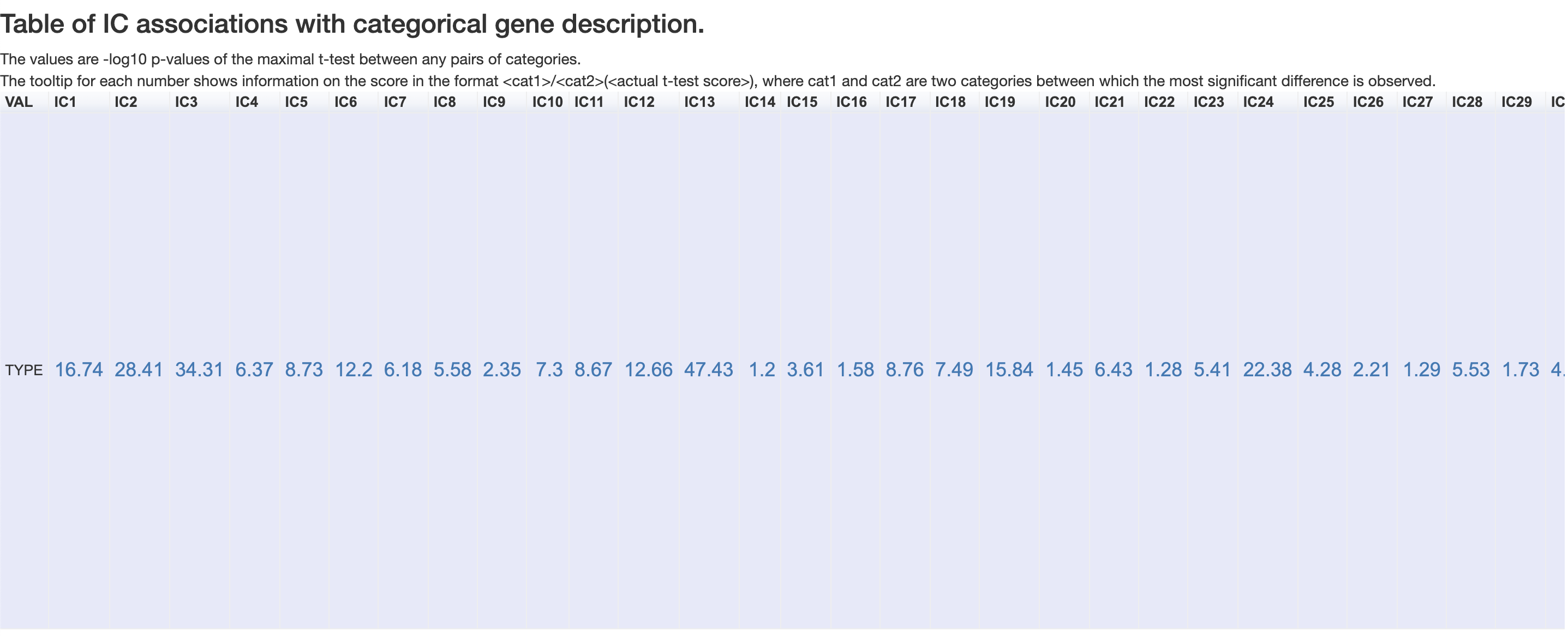
Clicking on the number of the IC13 shows the following charts:

We can see that ‘protein_coding’ and ‘snoRNA’ categories have the biggest difference between their means.
Association with numerical features
For a numerical gene annotation, its association with a metagene is computed by the Spearman correlation coefficient.
In this tutorial, GC-content is the only numerical gene annotation we have. IC26 has the highest correlation to GC-content, and it equals 0.19.

Associaion with known metagenes
The associations with previously known metagenes are computed with the Spearman correlation coefficient.

IC5 recieved a strong (0.62) correlation with a previously identified M7_CELLCYCLE. GSEA and ToppGene analyses from previous tutorials suggested a strong association of this metagene with genes involved in the process of cell cycle, generating the consistency of findings about this independent component.
